Servo control interface in detail

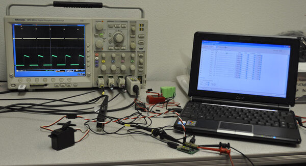
Last time, I gave a basic introduction to the simple pulse interface for sending commands to servos. In this post, I want to explore some of the details and ramifications of the servo interface in a bit more depth. I’ll be using the Mini Maestro 12-channel servo controller, which offers a lot of servo control flexibility, and a current probe with my oscilloscope to illustrate servos’ responses. Here’s the basic setup:

In this close-up picture, you can see that I have the current probe on a servo extension cable so that I can easily change servos without touching anything else:

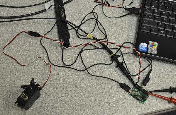The red and black clips in the lower-right corner go to a variable power supply, and the netbook has the Maestro Control Center software running on it to allow quick changes to the servo control pulse width and frequency.

Before we get to some screen shots, let’s go over the basic signal we’re sending to the servo. The signal is a square wave, meaning there are two voltage levels between which we switch instantly (in real life, the transition has to take some amount of time, but that transition time is so short that we can approximate it as zero):

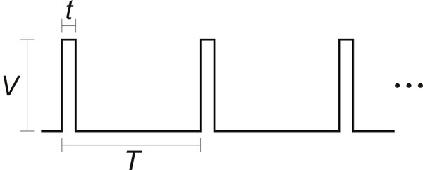The signal alternates between zero volts and the pulse voltage, so there are only three parameters necessary to characterize the waveform:

• Pulse voltage, V
• Pulse width, t
• Pulse period, T

Let’s consider each of these parameters.

Pulse voltage

As we saw in the RC receiver output signals from last time, the pulse voltage can vary quite a bit. Modern receivers have 3.0 V signals, but many servo controllers use 5.0 V or more. For the most part, this signal amplitude does not matter too much, as a long as it is high enough for the servo to register the pulses, and the valid range is perfect for interfacing directly to a microcontroller that is running at 3.3 V or 5.0 V. We put 220-ohm resistors in line with the outputs of our servo controllers, which run on approximately 5.0 V; the resistors protect the pins in general but also prevent too much current from flowing in the event that the servo is running at a lower voltage than the signal it is getting.

Pulse width

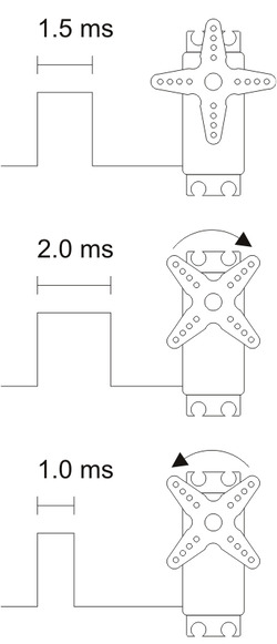The pulse width is generally the most important part of the interface, and that is what we intentionally vary to change the command to the servo. The general idea is simple: a pulse width of 1.5 ms is what we consider “neutral”; increasing the pulse width will make the servo go one way, and decreasing the pulse width will make the servo go the other way. However, there are a few points you should keep in mind:

• The neutral point is not necessarily the middle of the servo’s absolute maximum range. For instance, a servo that is capable of 180 degrees of movement might have the output at the 100-degree point for a 1.5 ms input pulse. In that case, the available range would be 80 degrees to one side of neutral and 100 degrees to the other. The pulse width that corresponds to the middle of the available range will vary from servo to servo, even for servos that are of the same model, so if you care about getting the most range you can and having neutral mean the middle of that range, you will have to calibrate your system for each servo.

• There is no standard correspondence between the pulse width and the servo position. Generally speaking, moving from 1.0 ms to 2.0 ms will yield about 90 degrees of servo movement, but that pulse width range could correspond to 100 degrees on one servo and 80 degrees on another servo. This means that any servo controller or servo control library you might use that makes any claims about absolute degrees is hiding something from you (or designed by someone who doesn’t really understand the interface). If you change servos in your design, you might have to make corresponding changes in the range of pulses you send to it, so if you are doing your own servo pulse generation, it’s a good practice to have the neutral point and range of your servo parametrized in your code. (I’ll cover more on that in a future post.)

• Similarly, there is no standard minimum and maximum pulse width. If you keep making the pulses wider or narrower, servos will keep moving farther and farther from neutral until they hit their mechanical limits and possibly destroy themselves. This usually isn’t an issue with RC applications since only about half of the mechanical range is ever used, but if you want to use the full range, you have to calibrate for it and be careful to avoid crashing the servo into its limit.

• The direction that a servo turns for increasing pulse widths is not standardized, either (also, it’s usually not specified). In my diagram to the right, I show the output moving clockwise as the pulse width increases, but that could easily be the other way around. We can expect the correspondence to stay consistent between different units of the same servo model, but the direction of servo travel is yet another thing you should be able to change in your design without a lot of effort so that you have the option of changing servo models.

• The servo control interface is an analog interface. The signals look digital because we have square waveforms and we use digital microcontroller outputs to create them, but because what matters is the infinitely variable time that the pulse is high, the signal is analog, and any slight jitter in the pulse width will cause corresponding twitching in the servo output.

• Although we can use some pulse width modulation (PWM) hardware modules in microcontrollers to generate servo control signals, and we are changing (modulating) the pulse width, it’s not good to call the signals PWM signals because that implies the relevance of the duty cycle, which is the percentage of on (high) time of the signal. As we will see next, the frequency of the pulse train does not affect the servo position if the pulse width stays the same, so changing the duty cycle does not necessarily affect the servo position. Similarly, we could keep the duty cycle constant by stretching out both t and T by the same proportional amount, and the servo position would change since the pulse width had changed.

Pulse period

The typical pulse period is around 20 ms, which corresponds to a frequency of 50 Hz. One immediate ramification of the pulse rate is that it gives you an upper bound on how quickly you can give the servo new commands. Most servos can handle substantially faster pulse rates, and some special servos are designed to support pulse frequencies of several hundred hertz. However, a more subtle dependence on the pulse frequency shows a major difference between analog and digital servos, and that will be the focus of most of the rest of this post.

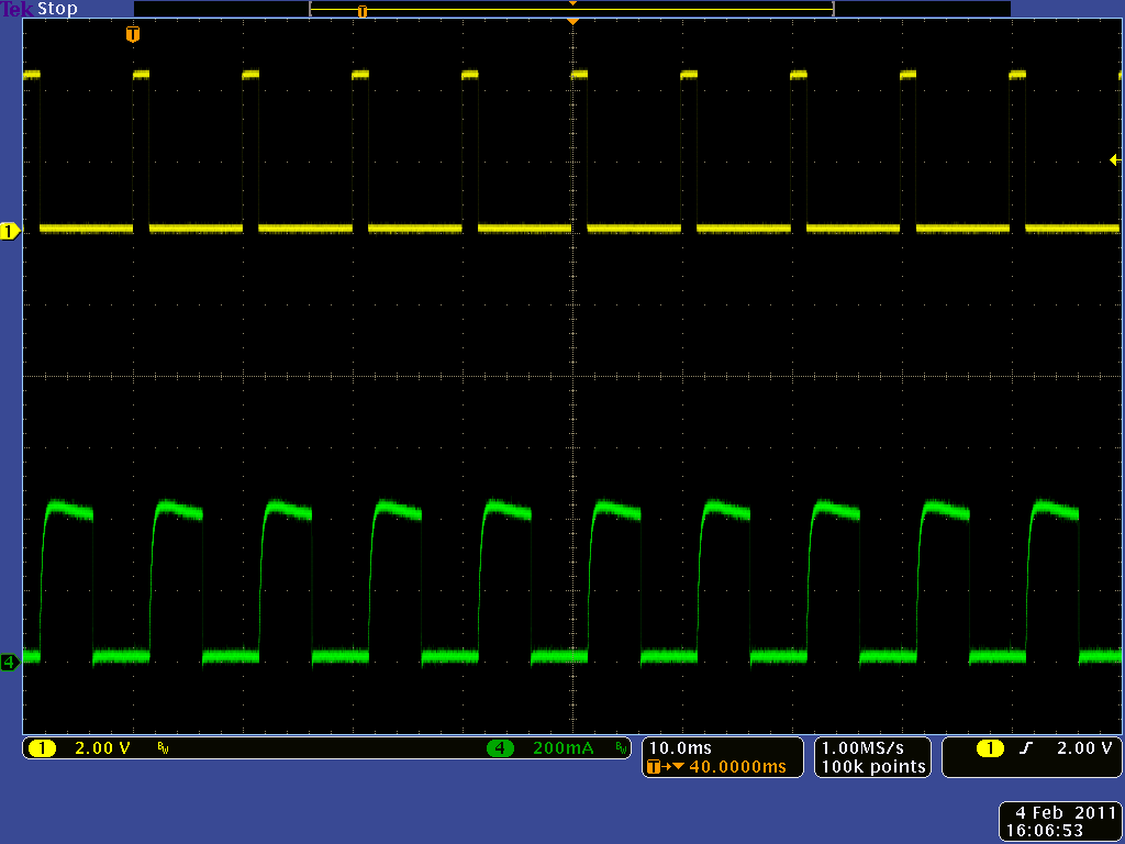
Here is the input signal and current consumed by a Futaba S148, a quintessential standard analog servo, connected to the setup I showed earlier:

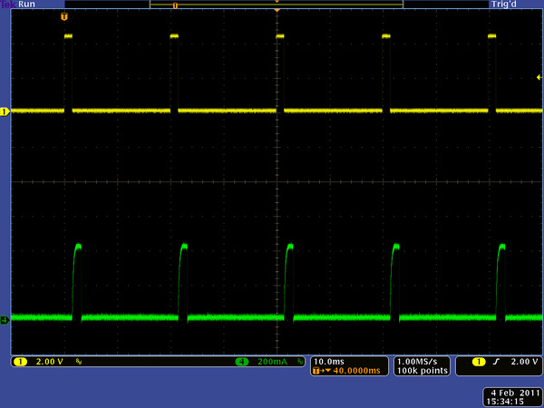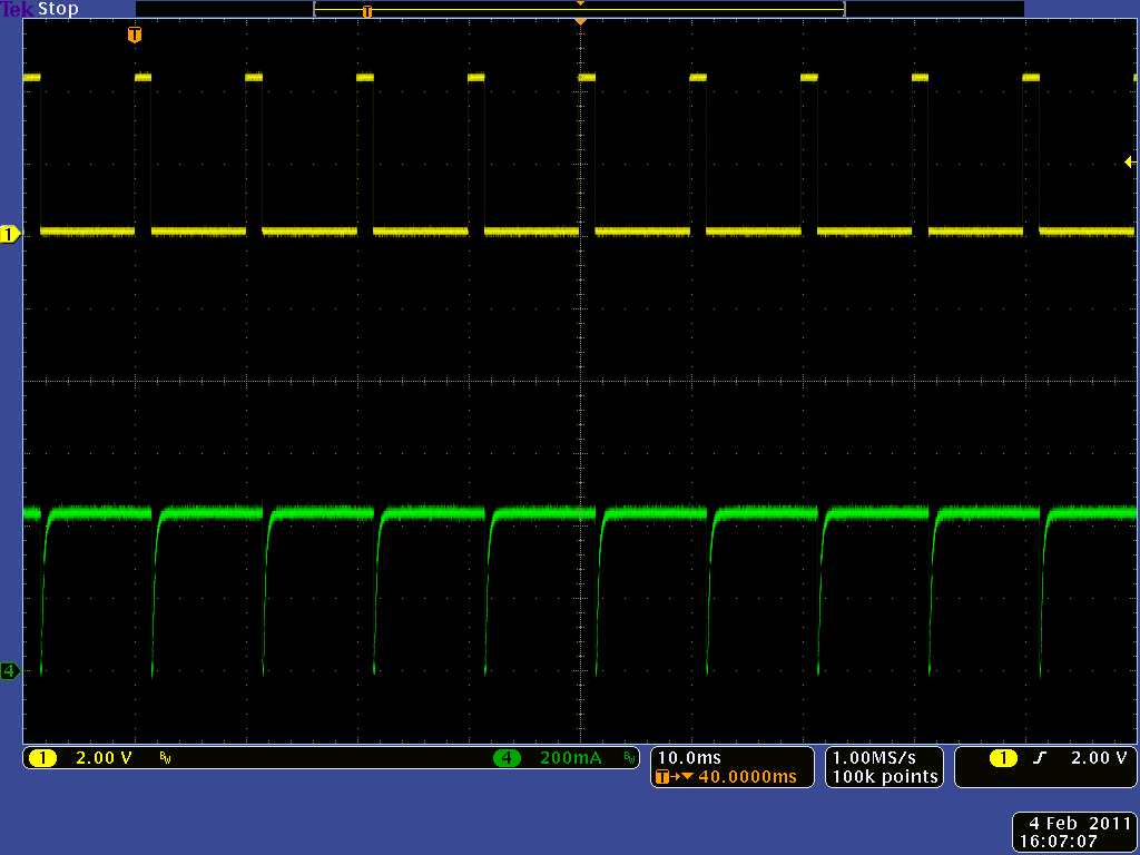
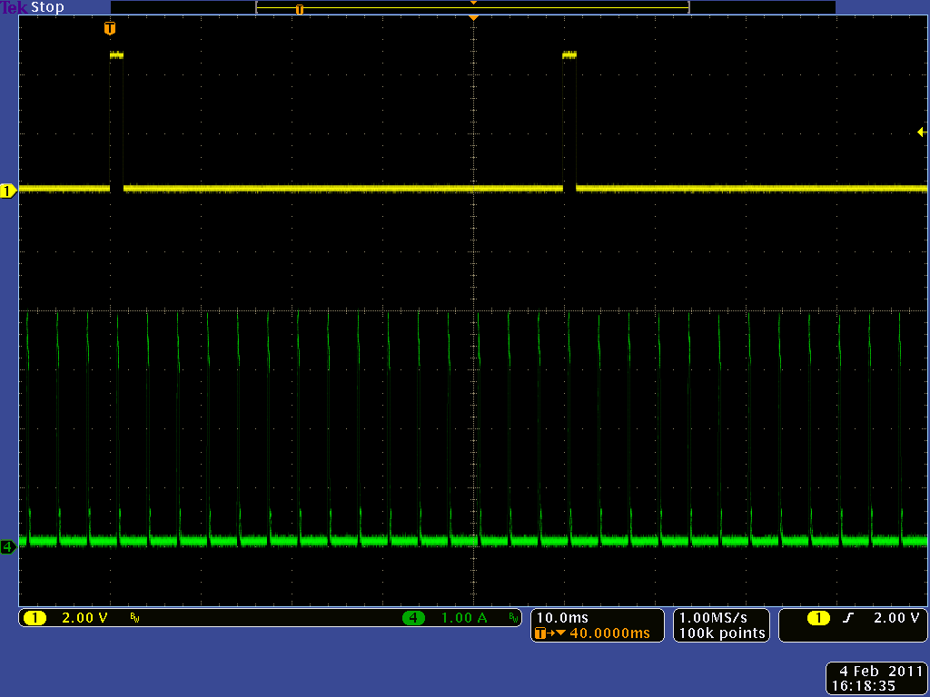
(The yellow trace on top is the control signal; the lower, green signal is the current used by the servo.) I was pushing slightly against the output shaft, and we can see that each command pulse is immediately followed by a pulse of current as the servo tries to push back against me. As I pushed harder, the servo pushes back for a longer time after each command pulse:

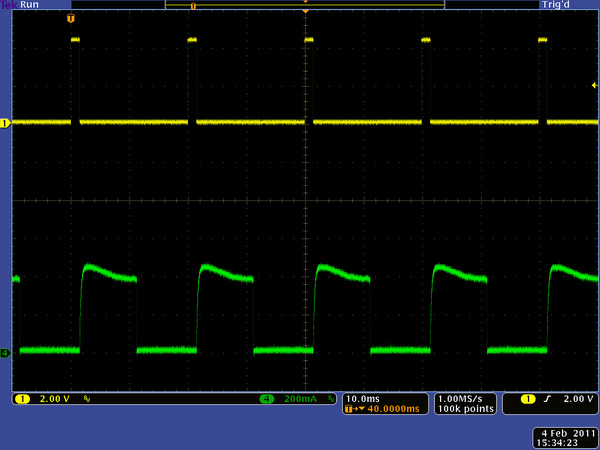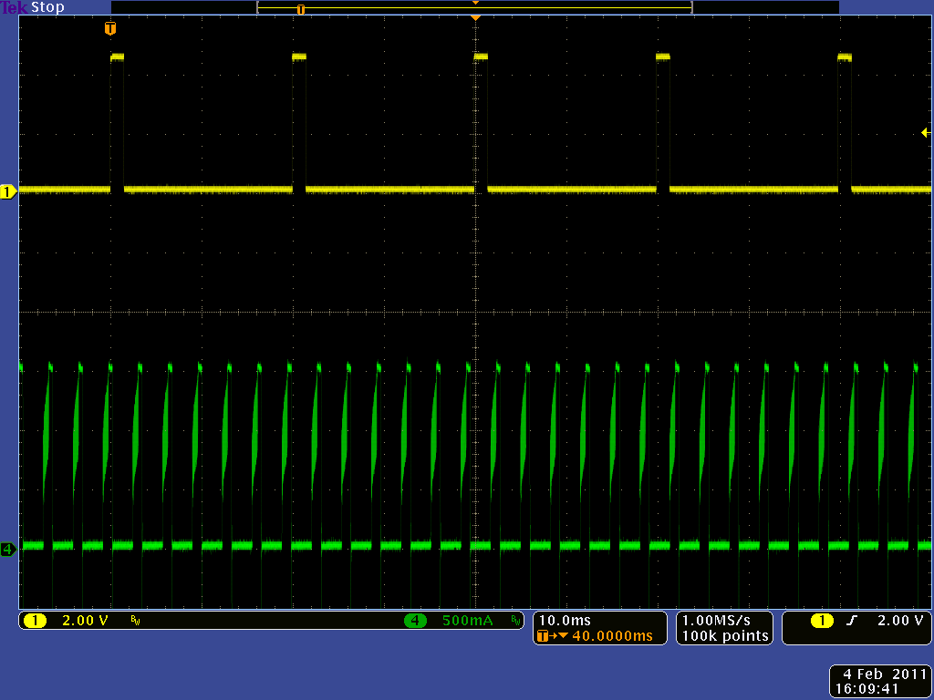
I had the power supply set to 3.5 V so that the servo could not push back as strongly as it could and possibly damage itself. If we reduce the pulse rate from 50 Hz to 20 Hz, we see that the current bursts also drop to 20 Hz:

Oscilloscope trace of S148 servo current with 20 Hz signal, 3.5 V supply, low mechanical load.

Oscilloscope trace of S148 servo current with 20 Hz signal, 3.5 V supply, high mechanical load.

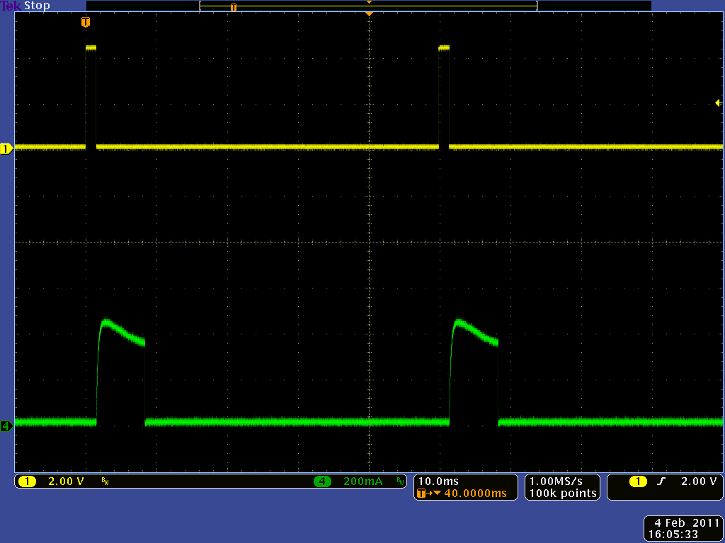
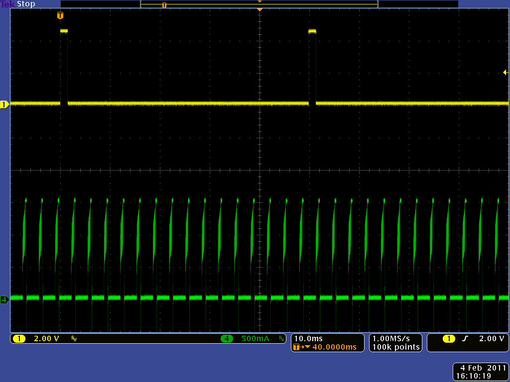
The servo still generally works at the lower pulse frequency, but the duty cycle (percentage of the time that it is pushing back) goes down so that its torque also goes down. As the pulse period gets even longer, the time between attempts to correct the servo position gets correspondingly longer, and at slow pulse rate like 10 Hz, the output torque has enough ripple that it is easy to feel. Shortening the pulse period has the opposite effect; at 100 Hz, the servo is pushing back almost 50% of the time even with a slight output resistance, and with a high mechanical load, the servo is pushing back almost 100% of the time:

Oscilloscope trace of S148 servo current with 100 Hz signal, 3.5 V supply, low mechanical load.

Oscilloscope trace of S148 servo current with 100 Hz signal, 3.5 V supply, high mechanical load.

A nice feature of this general operation of analog servos is that if you stop sending pulses, the servos will stop trying to hold a position and effectively turn off: they will no longer resist changes to the output position (whether they can mechanically handle backdriving is a separate issue) and reduce their current to the minimum idle value.

Digital servos have an internal microcontroller that allows the servo designers much more flexibility in how servos react. Next up, I have corresponding screen shots from a relatively high-performance digital servo, the GD-9257:

We see that the current pulses are much quicker than the control pulses; also, even with a slight output load, the peak current is past 1.5 A at only 3.5 V. At full voltage, the current peaks would be around 2.5 A, so we see that multiple servos can quickly become a very demanding load for a power supply. At a higher mechanical load, it is especially clear that the servo’s performance does not depend on the pulse frequency:

Oscilloscope trace of GD-9257 digital servo current with 50 Hz signal, 3.5 V supply, high mechanical load.

Oscilloscope trace of GD-9257 digital servo current with 20 Hz signal, 3.5 V supply, high mechanical load.

I tried various other servos, but they generally behaved the same way. One slightly more interesting unit was the DS8325HV high-voltage servo, which did not even operate at 3.5 V. At 5.0 V, the waveforms are similar to the earlier digital ones, but the current spikes are now up to 4 amps:

Oscilloscope trace of DS-8325HV digital servo current with 100 Hz signal, 5.0 V supply, high mechanical load.

Oscilloscope trace of DS-8325HV digital servo current with 20 Hz signal, 5.0 V supply, high mechanical load.

One of the most interesting distinctions among digital servos does not show up in screenshots: some digital servos continue holding the most recent position even if the control signal goes away, and other digital servos turn off. As usual with RC products, this behavior is not documented, and it can have important ramifications for robotics and other non-RC projects. For low-power applications, it’s great to be able to turn off a servo by not sending it control pulses. On the other hand, it can be nice to have a servo maintain its position if you have many servos to control and do not need to update their position often. For instance, if you have a 30-servo kinetic sculpture that does not need to move quickly, you could send each servo a separate command every ten seconds and comfortably generate each servo pulse separately; with analog servos or servos that turn off without a signal, you might be faced with the much more complicated task of generating simultaneous servo pulses.

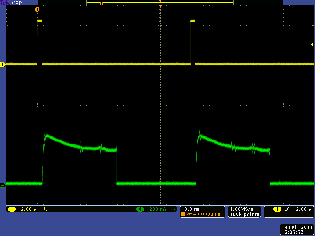
I have one final fun screen shot to show you. This is back to the S148 servo, but this time, the oscilloscope capture is over a longer period, as the servo is moving:

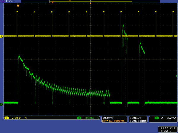The first control pulse on the left is for a new servo position, and we see the current jump up as the servo starts moving. There’s no mechanical load beyond just the servo, so the current goes down as the output speeds up. As the servo reaches its destination, it overshoots slightly and changes direction, which causes the current to spike up even higher than the initial starting current.

Conclusion (for now)

At this point, you should have a good idea about the range of reactions servos could have to the control signals we send them. Next time, I’ll move on to considerations of how to generate those signals.