5. Setting Up Your System

The following step-by-step procedure is recommended for configuring a feedback system for use with a jrk motor controller.

Connecting power and feedback

1. Connect your jrk to a PC with a USB cable and launch the configuration utility. The red LED should be on.
2. Select the “Reset to default settings…” option from the File menu to load a safe set of settings.
3. With your power supply off, make the power connections to VIN and GND.
4. Connect your feedback sensor to the FB input. If you are using a potentiometer as a feedback sensor, use the AUX pin to power it, and enable Detect disconnect with AUX in the Feedback tab.
5. Set the “No power”, “Motor driver error”, “Feedback disconnect”, and “Max. current exceeded” errors on the Error tab to Enabled and latched. This should stop your system in case of any major problem.
6. Click “Apply settings to device”.
7. Turn on power.
8. On the Error tab, click “Clear Errors” to remove the errors caused by turning off the power.

The red LED should now be off, and the yellow LED should be blinking slowly, indicating that the board has power but that no target has been set. If the red LED is on, examine the Errors tab to determine the source of the problem. Look at the value of Scaled Feedback displayed at the top of the window, and verify that it changes if you manually adjust the feedback sensor.

Calibrating feedback

1. Select the correct value for Feedback mode.
2. Click “Learn…” on the Feedback tab. You will be prompted to turn the output to its minimum and maximum positions, so that readings of the feedback sensor can be determined at each extreme.
3. Examine the resulting values and adjust if desired. Your system will be safer if you set Absolute Max. and Absolute Min. to values that the system can actually reach, so that if motion takes it past those extremes, the jrk will automatically shut down (because of the “Feedback disconnect” error.)
4. Click “Apply settings to device”.
5. Move the system to the middle of its range.

Setting motor limits

1. Set Max. duty cycle to a safe value, like 200.
2. Set Max. current to a safe value, like 500 mA. You want values that will turn the motor but not give it enough power to do any damage if something goes wrong.
3. Set other limits as necessary.
4. Click “Apply settings to device”.

Connecting the motor

From this point on, be prepared to shut down the system by clicking “Stop motor” or turning off your power supply if anything goes wrong and the limits and errors set previously fail to stop the motor.

1. Turn off power.
2. Connect your motor wires to the jrk’s A and B motor outputs. If possible, connect them so that positive voltage at A causes the motor to drive forward.
3. Turn on power.

Testing the motor

1. If possible, drive your motor with feedback disabled. To do this, make sure that the Feedback mode is set to none and use the controls on the Input tab to apply different duty cycles. Of course, this requires you to have a system that does not destroy itself when run without feedback.
2. On the Error tab, click “Clear Errors” to remove the errors caused by turning off the power.
3. On the Motor tab, click the “Detect Motor Direction” button. This will apply some power to the motor and measure the direction that feedback moves in response. If the motor is connected “reversed” with respect to your feedback sensor, then Invert motor direction will be checked.
4. Click “Apply settings to device” to apply any changes.

Testing basic feedback

1. In the PID tab, choose a Proportional Coefficient of 1 and leave the other two constants at zero. This will probably drive your motor at its maximum duty cycle, so make sure that this and other motor parameters are configured correctly.
2. Click “Apply settings to device”.
3. Use the slider on the Input tab to send various input values to your jrk, and see how it behaves.

If you did everything correctly, your feedback system should now be active, approximately following the target value.

Tuning the PID constants

Tuning PID constants is a complicated process that can be approached in many different ways. Here we will give a basic procedure that works for some systems, but you will probably want to try various different methods for finding the best possible values. You will want to have the Plots window open, displaying a nice view of the Error, Target, Scaled Feedback, and Duty Cycle. When setting the Integral Coefficient, it will also be useful to look at the value of the Integral.

1. Increase your Max. duty cycle, Max. current, and other limits to reasonable values for high-performance operation of your system.
2. Try increasing the Proportional Coefficient until you reach a point where the system becomes unstable. Note that the stability could be different at different target positions, so try the full range of motion when hunting for instability.
3. Decrease the value from the point of instability by about 40-50%. This is the first step of the Ziegler-Nichols Method.
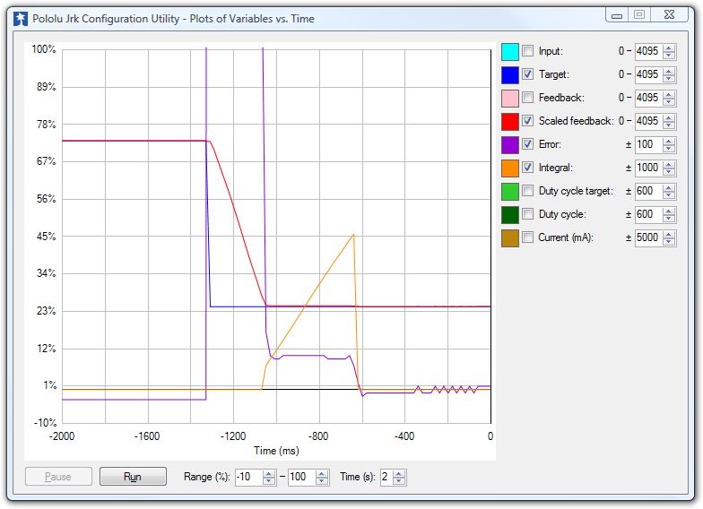
4. Note how close your system gets to an error of zero using just the proportional term. You can use the integral term to get it much lower: with the integral limit set at 1000, try increasing the Integral Coefficient until you see a correction that brings the error closer to zero. In the plot window shown here, you can see that the proportional term gets the error down to about 10, then the integral term builds up and, half a second later, moves the motor just a bit, reducing the error to ±1.
5. For systems that have a lot of friction relative to external forces, enable a Feedback dead zone so that the integral term doesn’t cause a slow oscillation very close to an error of zero. Watch how the integral term and duty cycle build up over time to achieve this. The plot was created with a dead zone of 4; without this, the integral term would have continued to build up, but at a slower rate, after the first adjustment.
6. Enable the Reset integral when proportional term exceeds max duty cycle option to prevent the integral from winding up during large motions. This is also shown in the plot: the integral term does not start increasing until the error is close to zero.
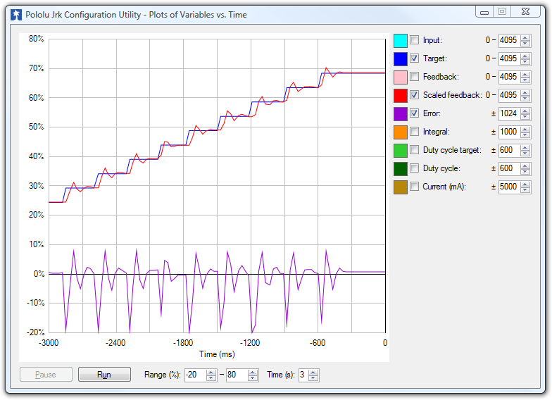
7. Have your system take large steps (for example, by clicking the bar area of the Input tab scrollbar to move the target by 200) and use the graph to examine whether it consistently overshoots (crosses zero before coming to a stop and moving back) or undershoots (does not reach zero before slowing down). The plot window shown here, drawn for a system using a Derivative Coefficient of zero, shows clear overshooting. In this example, the error actually oscillates back and forth several times before settling down.
   
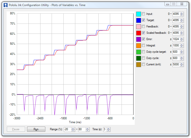
8. Increase the Derivative Coefficient to get rid of any overshooting, but not so much that it undershoots. The plot window shown here demonstrates undershooting, using a Derivative Coefficient of 10. You can see that the error never reaches zero. Instead, it gradually approaches zero after each step.
9. Experiment with your system. Adjust any parameters as necessary to get the behavior that you need.

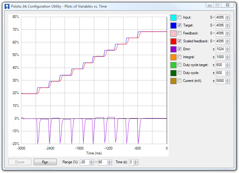
The following example plot shows a well-tuned system, with Proportional, Integral, and Derivative Coefficients of 6.0, 0.25, and 7.5. When taking steps, the system stops very quickly at a position with very small error, randomly overshooting or undershooting by a small amount.